Form V Data Variation: How to Explain Changes in Water, Raw Material, Pollution and Waste

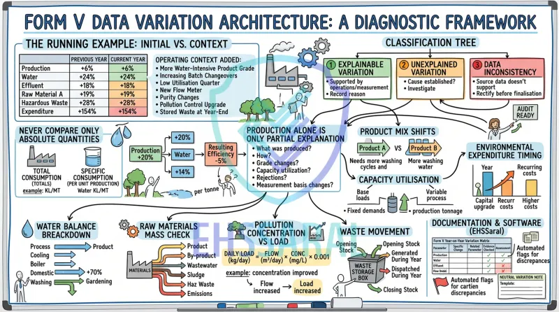
A Form V working sheet is nearly complete.

Production has increased by 6% compared with last year.

But water consumption has increased by 24%.

Effluent generation is up by 18%.

Hazardous-waste generation has increased by 28%.

Raw-material consumption per tonne of production is also higher.

At first glance, the figures look inconsistent.

But that does not automatically mean that anything is wrong.

In many Indian plants, environmental numbers do not move in exactly the same proportion as production. Product mix changes. Plants operate at different utilisation levels. More cleaning may be required. New meters get installed. Old estimates are replaced with actual measurements. Waste generated in one year may be dispatched in another.

The important question is therefore not:

“Why doesn't this year's Form V match last year's?”

The better question is:

“Can the change from last year to this year be explained by the underlying operations and supported by records?”

That distinction is important because Form V itself is designed to bring together environmental information covering resource consumption, pollution and waste. The Environmental Statement is prescribed under Rule 14 of the Environment (Protection) Rules, 1986, for the financial year ending 31 March.

This article does not explain how to file Form V or how to collect its data department by department. Instead, it focuses on what should happen after the numbers are available but before they are accepted without question.

To know more on how to prepare Form V Environmental Statement

A Running Example: One Plant, Several Unusual Changes

Consider an anonymised multiproduct manufacturing plant.

Its current-year comparison looks like this:

If these figures are reviewed only as totals, almost every line appears to require an explanation.

But once the operating context is added, the picture may look very different.

During the year:

• the plant produced more of a water-intensive product grade;
• batch changeovers increased;
• equipment washing therefore increased;
• production ran at low utilisation during one quarter;
• a new calibrated water meter replaced an older estimation method;
• raw-material purity changed;
• a pollution-control upgrade was completed;
• and some hazardous waste generated late in the year remained stored at year-end.

Now the question is no longer whether the numbers “match.”

The task is to establish which variations are reasonable, which require investigation, and which indicate a data inconsistency.

1. First Classify the Difference: Variation, Unexplained Variation or Data Inconsistency

One of the most useful ways to review Form V data is to put every significant year-on-year change into one of three buckets.

For example:

Explainable variation

Production increased 20%.

Water increased 14%.

Water consumption per tonne actually reduced.

There may be little concern because the absolute increase is supported by higher activity and the specific consumption improved.

Unexplained variation

Production increased only 2%.

Water increased 25%.

There may still be a valid reason, but it deserves investigation.

Data inconsistency

The Form V working sheet shows annual water consumption increasing 25%.

But the monthly water-meter register shows only a 6% increase.

Now the issue is not simply variation.

There may be a calculation, transcription, unit-conversion or source-data problem.

This distinction prevents EHS teams from treating every large change as a problem - while also preventing genuine inconsistencies from being dismissed as “operational variation.”

Read building monthly Form V data readiness

2. Never Compare Only Absolute Quantities

This is where confusion often starts.

Suppose a plant reports:

Someone looking only at annual totals may say:

Water consumption has increased by 2,800 KL.

That is correct.

But it does not tell us whether environmental efficiency improved or deteriorated.

Now calculate water consumption per unit of production:

Previous year

20,000 KL ÷ 10,000 MT = 2.00 KL/MT

Current year

22,800 KL ÷ 12,000 MT = 1.90 KL/MT

So:

• absolute water consumption increased by 14%;
• production increased by 20%;
• specific water consumption actually decreased by 5%.

The plant used more water overall because it produced more.

But it used less water for every tonne produced.

That is a very different conclusion.

Absolute quantity and specific consumption answer different questions

Absolute quantity tells us:

What was the plant's total environmental footprint?

Specific consumption tells us:

How much resource or pollution was associated with each unit of production?

Both matter.

A useful Form V year-on-year review should therefore compare both wherever the data allows.

The same principle applies to:

• water per MT of product;
• raw material per MT;
• fuel per MT;
• effluent per MT;
• hazardous waste per MT;
• sludge per KL of effluent treated;
• or another meaningful production denominator.

3. Production Alone Does Not Explain Environmental Performance

It is tempting to compare every environmental parameter directly with total production.

Production +10%?

Then water, waste and raw-material consumption should also be around +10%.

In day-to-day operations, factories rarely behave so neatly.

Total tonnes are only one part of the explanation.

A meaningful variation review should also ask:

• What was produced?
• How was it produced?
• How many batches were run?
• How many grade changes occurred?
• What was the plant's capacity utilisation?
• Were there shutdowns or commissioning periods?
• Did rejection or reprocessing increase?
• Did the measurement basis change?

These questions often explain more than annual production volume alone.

Product Mix Can Change Environmental Intensity

Consider a plant producing two products.

Product A

Requires relatively little process water and one final wash.

Product B

Requires additional reaction water, multiple wash cycles and more equipment cleaning between batches.

Last year:

• Product A = 80%
• Product B = 20%

This year:

• Product A = 55%
• Product B = 45%

Total production might increase by only 6%.

But water consumption could reasonably increase much more.

Effluent may rise.

ETP chemical consumption may rise.

Sludge generation may also rise.

The annual production number alone cannot explain this.

Product grade can matter even when the product name remains the same

The issue is not limited to completely different products.

Different grades of the same product may require:

• different raw-material ratios;
• longer washing;
• additional purification;
• solvent recovery;
• different temperatures;
• additional filtration;
• more batch changeovers.

For multiproduct pharmaceutical, chemical, speciality-chemical, food, coating and similar plants, this becomes particularly important.

Same annual tonnage does not necessarily mean the same environmental load.

4. Shutdowns, Trials and Capacity Utilisation Can Distort Per-Unit Numbers

Suppose a plant normally produces 1,000 MT every month.

During one year, major maintenance and market conditions reduce production significantly.

For several months, however, the factory still requires:

• cooling-tower circulation;
• boiler warm-up;
• minimum scrubber operation;
• domestic water;
• utility water;
• lighting;
• ETP/STP operation;
• periodic equipment washing.

These environmental demands do not necessarily fall to zero when production falls.

This creates an important distinction between base load and variable process load.

This is why a low-production year can show worse specific consumption.

For example:

Normal year

Production = 12,000 MT
Water = 24,000 KL
Specific consumption = 2.0 KL/MT

Low-utilisation year

Production = 7,000 MT
Water = 18,000 KL
Specific consumption = 2.57 KL/MT

Total water actually decreased.

But water per tonne increased by almost 29%.

That does not automatically establish poorer operating discipline.

The fixed or semi-fixed environmental demand is now spread across fewer tonnes of production.

The plant should still investigate the movement, but the capacity-utilisation context matters.

Trial Production and Commissioning Can Have the Opposite Effect

A commissioning period can consume resources without producing normal saleable output.

There may be:

• trial batches;
• flushing;
• line cleaning;
• off-specification material;
• start-up losses;
• repeated adjustments;
• additional sampling;
• wastewater generation.

Specific consumption during such a period can therefore appear unusually high.

If the annual Form V figure includes such months, the EHS team should understand their contribution rather than comparing only the annual totals.

5. Measurement Changes Can Create an Apparent Environmental Change

Not every year-on-year change represents a physical change in the plant.

Sometimes the plant simply measured something better this year.

That difference matters.

Meter replacement

Suppose water consumption was historically estimated using pump operating hours.

A calibrated flow meter is installed this year.

The new measurement shows water consumption 17% higher than previous estimates.

Has water consumption actually increased?

Possibly.

But another possibility is that the previous estimation method understated consumption.

The two years are therefore not directly comparable without noting the measurement change.

Meter calibration drift

An existing meter may gradually over-record or under-record flow.

After calibration or replacement, the reported annual quantity may shift.

A sudden year-on-year variation should therefore sometimes lead back to:

• meter calibration certificates;
• meter replacement dates;
• opening and closing readings;
• breakdown periods;
• estimated values used during meter failure.

New meters can expose previously hidden streams

A plant may initially have one common water meter.

Later it installs separate meters for:

• process;
• cooling;
• domestic use;
• boiler feed;
• gardening;
• recycled water.

The newer data can be more accurate but less comparable with historical estimates.

That is not a reason to force the new figure to look like the old one.

It is a reason to document the change in measurement basis.

Estimation methodology can also change

Typical examples include:

• tanker quantity previously based on nominal tanker capacity, now based on actual receipts;
• production previously reported as gross production, now based on finished product;
• waste previously estimated from container count, now based on weighbridge data;
• fuel based on purchase quantity versus actual issue/consumption;
• liquid quantity converted from kilograms using an updated density;
• laboratory reporting method changed.

A good variation review therefore asks:

Did the environmental performance change, or did the way we measure environmental performance change?

Sometimes the answer is both.

6. Water and Effluent Variation Should Be Read as One Physical Story

Water is one of the most common areas where Form V figures look different from the previous year.

Suppose our example plant shows:

• Production: +6%
• Water consumption: +24%
• Effluent generation: +18%

A simple comment saying “water increased because production increased” is not sufficient.

The production movement does not explain the full increase.

The next step is to understand where the additional water went.

Break total water into its major uses

For example:

Now the variation starts becoming understandable.

The largest abnormal increase is in equipment washing, not process water.

A review of operating records may show that the number of product-grade changeovers increased substantially during the year.

Now the environmental variation has an operational explanation.

Effluent does not have to increase in exactly the same proportion as water

Water entering a plant can leave through several routes.

Depending on the process, it may become:

• process wastewater;
• domestic sewage;
• cooling-tower evaporation;
• boiler losses;
• product moisture;
• recovered or recycled water;
• gardening use;
• evaporation;
• sludge moisture;
• other legitimate losses or uses.

So if water increases 20%, effluent does not necessarily have to increase 20%.

The relationship should, however, make physical sense.

Example A

Water +20%
Effluent +5%

Possible reasons could include greater cooling-water demand, gardening, evaporation or increased reuse.

Example B

Water +5%
Effluent +25%

Now the EHS team may need to examine:

• increased washing;
• RO reject;
• boiler/cooling blowdown;
• process-water distribution;
• rainfall ingress where relevant;
• changed flow measurement;
• estimated versus metered quantities.

The purpose is not to manipulate the water balance until it looks perfect.

The purpose is to understand where the water physically went.

7. Raw-Material Consumption per Unit of Production: Ask Where the Material Went

Raw-material variation becomes much more meaningful when considered on a production-normalised basis.

Return to our example plant.

Production increased 6%.

Raw Material A increased 19%.

That difference deserves a closer look.

Suppose:

Previous year

Raw Material A = 5,000 MT
Production = 10,000 MT

Specific consumption:

0.50 MT raw material/MT product

Current year

Raw Material A = 5,950 MT
Production = 10,600 MT

Specific consumption:

0.561 MT/MT product

Specific consumption has increased by approximately 12%.

The useful question now becomes:

Why does the plant require more Raw Material A for each tonne of output?

Potential explanations include:

• product-mix change;
• different formulation;
• lower raw-material purity;
• moisture variation;
• reduced process yield;
• additional rejects;
• increased reworking;
• start-up losses;
• trial production;
• changed production denominator;
• inventory accounting differences;
• reduced recovery or reuse.

Use mass balance as a reasonableness check

When significant additional material enters a process, it generally has to appear somewhere in the system.

Depending on the process, material may end up as:

• finished product;
• intermediate;
• by-product;
• recovered material;
• wastewater;
• sludge;
• solid or hazardous waste;
• air emission;
• evaporation or moisture;
• rejects/rework;
• inventory.

Suppose Raw Material A consumption per tonne increases 12%.

But:

• product composition is unchanged;
• waste generation is unchanged;
• effluent load is unchanged;
• recovery is unchanged;
• rejects are unchanged;
• inventory is unchanged.

That does not prove the raw-material figure is wrong.

But it is a strong reason to look again.

There may be:

• a production-data issue;
• a stores/ERP boundary difference;
• an unrecorded loss;
• an inventory movement;
• or a measurement/definition change.

Environmental data becomes more reliable when related quantities are examined as a connected system rather than as independent spreadsheet cells.

8. Pollution Concentration Can Improve While Pollution Load Increases

This is one of the most commonly misunderstood environmental comparisons.

Suppose an ETP's COD concentration changes as follows:

Previous year

Average effluent flow = 100 m³/day
COD concentration = 500 mg/L

Current year

Average effluent flow = 150 m³/day
COD concentration = 400 mg/L

At first glance, COD has improved because concentration reduced from 500 mg/L to 400 mg/L.

That conclusion is only partly correct.

The concentration is lower.

But more wastewater is being discharged.

Simple pollution-load calculation

For an approximate daily load:

Pollution load (kg/day) = Flow (m³/day) × Concentration (mg/L) × 0.001

Previous year:

100 × 500 × 0.001
= 50 kg COD/day

Current year:

150 × 400 × 0.001
= 60 kg COD/day

So:

• COD concentration reduced by 20%;
• but estimated COD load increased by 20%.

Both statements can be true at the same time.

Why this matters for Form V variation analysis

A year-on-year comparison should therefore avoid statements such as:

“COD reduced by 20%, therefore pollution reduced by 20%.”

That may not be correct if the effluent flow changed.

Instead, examine:

Concentration + Flow = Load

The same logic can be applied, where appropriate, to parameters such as:

• BOD;
• COD;
• TSS;
• other measured pollutants.

For annual comparison, operating/discharge days and the actual basis used for annualisation also matter.

The important point is conceptual:

Concentration tells us how strong the pollutant is in a given volume. Pollution load tells us how much pollutant is being released over a period.

One cannot automatically substitute for the other.

9. Waste Generation, Waste Dispatch and Closing Stock Can Move Differently

Another frequent source of confusion is comparing waste generation with waste dispatched.

These are not necessarily the same quantity during a financial year.

Consider:

Someone may ask:

How did the plant dispatch 53 MT when it generated only 50 MT?

Because 8 MT was already present at the beginning of the year.

Similarly, a plant may generate 50 MT but dispatch only 42 MT because some quantity remains stored at year-end.

For variation analysis, the basic relationship is:

Opening stock + generation − dispatch/other legitimate movement = closing stock

This article deliberately stops at that conceptual level.

Detailed hazardous-waste reconciliation is a separate exercise involving the underlying statutory records, manifests, acknowledgements and disposal evidence. Where the issue is specifically a waste mismatch, refer to EHSSaral's dedicated guidance on reconciling Form 3 register entries with Form 10 manifest acknowledgements rather than trying to resolve the entire chain inside the Form V variation analysis.

Learn why Form IV and Form V waste figures can differ

Waste generation per tonne can still reveal useful information

Suppose:

Production +6%

Hazardous-waste generation +28%

That is worth examining.

Possible reasons could include:

• different product mix;
• more off-spec production;
• additional cleaning;
• ETP sludge variation;
• disposal of obsolete material;
• maintenance activity;
• contaminated containers;
• changed waste classification;
• better measurement;
• commissioning activity.

Again, the software or comparison table can identify the exception.

The EHS professional still needs to establish the reason.

10. Environmental Expenditure Can Change Sharply Without Indicating a Compliance Problem

Environmental expenditure is different from water or raw-material consumption because it is often affected by timing.

Consider this three-year example:

Looking only at the percentages could lead to strange conclusions.

Expenditure first increases sharply and then falls sharply.

But the underlying story is straightforward.

One year included a major capital project.

The following year did not.

Environmental expenditure may include different combinations of:

• routine monitoring;
• ETP/STP operation;
• pollution-control equipment maintenance;
• environmental laboratory work;
• hazardous-waste disposal;
• consultancy;
• instrumentation;
• capital upgrades;
• monitoring equipment;
• improvement projects.

The useful year-on-year question is therefore:

What changed in the environmental activities or capital programme?

A lower expenditure number does not by itself establish reduced environmental performance.

Likewise, a higher expenditure number does not automatically establish improved performance.

The nature of the expenditure matters.

11. Build a Form V Year-on-Year Variation Matrix

Rather than reviewing each number informally, a simple comparison matrix can make the process much more disciplined.

A useful structure is:

*Illustrative figures only; the actual annual load should be calculated using the plant's appropriate monitoring, flow and operating-period basis.

The most important columns are not necessarily the percentages.

They are:

Related parameter
and
Evidence checked

Those two columns force the reviewer to ask whether the explanation is supported by something beyond memory.

12. Compare Four Things, Not Just This Year Against Last Year

A strong Form V variation review can examine each important parameter at four levels.

1. Absolute year-on-year movement

Example:

Water:

20,000 KL → 24,800 KL

Change:

+24%

This tells you the scale of the movement.

2. Production-normalised movement

Production increased only 6%.

So water per MT also increased.

This tells you whether the plant's environmental intensity changed.

3. Monthly pattern

Did water gradually increase throughout the year?

Or did almost the entire increase occur between April and June?

This matters.

A three-month spike may point toward:

• shutdown/restart activity;
• commissioning;
• meter replacement;
• leakage;
• abnormal washing;
• trial production.

An annual total can hide this completely.

4. Related-parameter movement

If water increased, what happened to effluent?

If raw-material consumption increased, what happened to production yield?

If effluent concentration fell, what happened to total load?

If waste increased, what happened to production mix?

This fourth comparison is where environmental data becomes particularly useful.

Instead of reviewing isolated figures, the plant starts reviewing relationships.

13. What Percentage Variation Should Trigger an Investigation?

This is one of the first questions EHS professionals ask.

Should anything above 10% be investigated?

20%?

25%?

There is no sensible universal percentage that can be applied to every environmental parameter and every factory.

A useful internal exception rule should consider several factors together.

Percentage movement

A 30% change naturally attracts attention.

But percentage alone can mislead.

Moving from 1 kg to 1.3 kg is also a 30% increase.

Absolute materiality

A small percentage change in a very large water-consumption figure may represent a significant quantity.

Production-normalised movement

Water +20% with production +25% is different from water +20% with production unchanged.

Proximity to consent or other applicable limits

A relatively small movement may deserve attention where a parameter is already close to an applicable limit.

Historical variability

Some parameters naturally move considerably with product mix or seasonal operation.

Others are normally very stable.

Measurement reliability

A large change from an estimated historical figure to a new calibrated measurement should be interpreted differently from a large change measured using an unchanged system.

Environmental significance

Plants may also integrate these internal exception criteria with their broader environmental-management-system approach to identifying significant environmental performance changes.

The objective is not to create an artificial regulatory threshold.

The objective is to ensure that material and unusual changes do not pass through Form V preparation without being understood.

14. How EHSSaral Can Surface Exceptions Before Annual Form V Finalisation

This is where Form V automation can go beyond generating a form.

A form-generation system can take approved annual numbers and place them into the required fields.

That is useful.

But the more valuable question is:

Which of those numbers should an EHS professional look at before the form is finalised?

EHSSaral can compare current environmental information against connected operational references such as:

• previous Form V figures;
• monthly production;
• water records;
• effluent records;
• monitoring results;
• waste-generation records;
• applicable consent information.

Instead of waiting for someone to manually compare two annual spreadsheets, the system can surface exceptions such as:

Water consumption increased 24%, while production increased only 6%.

Or:

Specific raw-material consumption increased 12% compared with the previous year.

Or:

Effluent generation increased 18%, while total water consumption increased 24%. Review the changed water-use distribution.

Or:

COD concentration decreased, but estimated pollution load increased because effluent volume increased.

Or:

Hazardous-waste generation increased 28%, while production increased 6%.

The important point is that the software should not automatically decide that these changes are wrong.

It should say:

This relationship deserves attention.

The EHS professional then investigates the plant-specific reason.

That distinction matters.

Software surfaces the exception.
Operations explain it.
Evidence supports the conclusion.

Catching variation earlier is more useful than discovering it at year-end

Imagine that water consumption starts rising disproportionately in November.

A monthly comparison shows:

Production: +4%
Water: +21%

If the change is noticed then, the EHS team can still examine:

• the meter;
• individual water streams;
• abnormal washing;
• utility performance;
• leakage;
• product mix;
• operating records.

If the same issue is noticed only while preparing the annual environmental statement months later, identifying the operational cause becomes harder.

People forget.

Shift records become difficult to trace.

Operational context gets lost.

That is why EHSSaral's longer-term value is not simply producing Form V.

It is creating continuity between monthly environmental records and annual environmental interpretation.

15. How to Write a Neutral, Evidence-Backed Variation Note

Not every variation needs a lengthy report.

For material or unusual changes, however, a short internal variation note can be useful.

Its purpose is straightforward:

Explain what changed, why the plant believes it changed, and what evidence was reviewed.

It should not sound defensive.

It should not try to “justify” a number that has not been verified.

It should simply document the reasoning.

A practical variation-note structure

Parameter:
[Environmental parameter being reviewed]

Observed variation:
[Previous-year figure] to [current-year figure], representing approximately [X%] change.

Production / activity movement:
[Relevant production, operating-day, batch-count or activity movement]

Reason investigated:
[Operational or measurement reason identified]

Evidence reviewed:
[List of supporting records]

Assessment:
[Explainable variation / further investigation required / data correction required]

Follow-up action, if any:
[Monitoring, verification or corrective action]

Example: Water-consumption variation note

Parameter: Total water consumption

Observed variation: Water consumption increased from 20,000 KL to 24,800 KL, representing an increase of approximately 24% compared with the previous reporting year.

Production movement: Total production increased approximately 6%.

Reason investigated: The additional increase was primarily associated with a higher proportion of Product B, increased product-grade changeovers and additional equipment-washing activity during the year. A water-meter replacement also improved measurement of one utility stream that had previously been partly estimated.

Evidence reviewed: Monthly water-meter records, production summary, batch/changeover records and meter-replacement/calibration documentation.

Assessment: Variation considered operationally explainable. Specific water consumption remains higher than the previous year and will continue to be reviewed through monthly monitoring.

This is much stronger than writing:

“Water increased due to production.”

The longer explanation shows that someone actually looked at the underlying cause.

Keep the variation note as part of the supporting compliance record

If management, an auditor, consultant or regulatory officer later asks why a reported parameter changed materially, the EHS team should be able to trace the number back to its operational reason and supporting records.

A good note does not guarantee that no further questions will arise.

But it gives the plant a clear internal record of how the figure was evaluated.

That is good compliance practice irrespective of who later reviews the data.

16. What If Last Year's Form V Figure Was Wrong - or Simply Not Comparable?

Sometimes a current-year variation investigation produces an uncomfortable conclusion:

This year's figure may actually be more reliable than last year's figure.

Several situations can cause this.

Previous year was based on estimation

This year uses calibrated measurement.

The values may not be directly comparable.

Reporting boundaries changed

Perhaps a water stream, waste stream or production line was excluded from the previous calculation but included this year.

Different denominator was used

Last year:

Gross production.

This year:

Finished saleable production.

Specific-consumption comparisons will be distorted.

Unit conversion was incorrect

Common possibilities include:

• kilograms versus tonnes;
• litres versus kilolitres;
• m³ versus KL;
• monthly versus annual values;
• density conversion;
• concentration versus total load.

Spreadsheet formula was incorrect

A copied formula may have omitted a month or referenced the wrong cell.

This can remain unnoticed until a year-on-year comparison exposes it.

Do Not Change Correct Current-Year Data Merely to Preserve Continuity

This is an important principle.

If the underlying current-year records support a figure, it should not be artificially altered merely because it differs sharply from the previous year's submission.

Instead, first determine what has changed:

Scenario 1: Comparability problem

Both figures may be reasonable, but they were produced using different methods or reporting boundaries.

Document the methodology difference.

Scenario 2: Possible previous reporting error

The evidence suggests that the earlier submitted number itself may have been incorrect.

This requires more care.

The plant should establish the historical position internally and determine, through the appropriate compliance function and where necessary in consultation with the concerned SPCB/PCC, whether any clarification or corrective submission is appropriate.

There is no value in creating a second questionable figure simply to make two years look consistent.

17. A Practical Form V Variation Review - Putting It All Together

Return to our original plant.

The first review showed:

After investigation:

Water +24%

Finding: Product B share increased and required more washing. Grade changes also increased. A new water meter improved measurement.

Assessment: Explainable variation, but specific consumption remains higher and deserves continued monitoring.

Effluent +18%

Finding: Increased washing contributed additional process wastewater. Water increased more than effluent because cooling-water use also increased.

Assessment: Explainable variation.

Raw Material A +19%

Finding: Specific consumption increased approximately 12%. Product B requires a higher proportion of Raw Material A and raw-material purity was slightly lower during part of the year.

Assessment: Explainable, subject to confirmation from production and stores records.

COD concentration -12%

Finding: ETP outlet concentration improved.

But because total effluent quantity increased, the change in annual pollution load was smaller than the concentration change alone suggests.

Assessment: Compare concentration and annual load separately.

Hazardous waste +28%

Finding: Higher Product B share and increased ETP sludge generation contributed to additional waste.

Assessment: Explainable only after checking the waste stream and underlying generation records.

Environmental expenditure +154%

Finding: Current year included a one-time pollution-control system upgrade.

Assessment: Timing/CAPEX-driven variation.

The final Form V numbers have not been made artificially smoother.

Nothing has been changed merely to resemble last year.

Instead, the plant now understands why the environmental profile changed.

That is the real purpose of year-on-year variation analysis.

18. Before Finalising a Materially Changed Form V Figure, Ask These Questions

Use this as a final diagnostic review.

• Has total production changed?
• What happens when the parameter is calculated per unit of production?
• Has product mix or product grade changed?
• Did the number of batches or changeovers change?
• Were there shutdowns, trial production or commissioning periods?
• Did plant capacity utilisation change materially?
• Does the parameter contain a fixed or semi-fixed environmental base load?
• Did any meter, laboratory method or estimation methodology change?
• Does the monthly pattern support the annual total?
• If water changed, does the water–effluent relationship make physical sense?
• If raw-material intensity changed, can the material movement be explained through yield, recovery, waste, effluent, emissions, rejects or inventory?
• If pollutant concentration changed, what happened to total flow and pollution load?
• Has waste generation been separated from dispatch and storage?
• Is environmental expenditure affected by a one-time capital project?
• Are current and previous years genuinely comparable?
• Have supporting records been checked?
• Is the variation explainable, unexplained or a data inconsistency?

If these questions can be answered clearly, the Form V figures become much easier to understand.

If they cannot, the unresolved variation is telling the plant where to look next.

Quick Summary

A Form V figure does not become questionable simply because it is different from last year.

What matters is whether the movement makes sense.

A strong year-on-year review should look at:

Absolute quantity → Specific consumption → Monthly pattern → Related environmental parameters → Supporting evidence

Production alone may not explain a variation.

Product mix, utilisation, shutdowns, cleaning frequency, measurement changes, water balance, pollution load, waste storage and capital expenditure can all change annual figures.

And where the underlying relationship does not make sense, the plant should investigate the data rather than invent an explanation.

This is also where environmental compliance software can become more useful.

Generating Form V is one task.
Knowing which Form V number deserves attention is a different capability.

EHSSaral is being designed around that second problem - connecting operational environmental records, comparing them with historical values and surfacing exceptions so that the EHS professional can investigate the right issue.

Good compliance starts with understanding what the numbers are saying.

Final Thought

The objective of a Form V year-on-year comparison is not to make this year's environmental statement look similar to the previous one.

Factories change.

Production changes.

Processes change.

Measurements improve.

Environmental loads move.

What matters is whether the plant understands those movements.

A number that changed and can be explained is very different from a number that changed and nobody knows why.

That is where meaningful environmental compliance intelligence begins.

Frequently Asked Questions

1. Why are my Form V figures different from last year's environmental statement?

Form V figures can change because of production volume, product mix, plant utilisation, raw-material quality, process changes, water use, shutdowns, trial production, waste generation, capital expenditure or changes in measurement methodology.

A difference is not automatically an error. The important question is whether the variation can be explained from underlying operational and environmental records.

2. What percentage of Form V year-on-year variation requires investigation?

There is no universal percentage that should automatically be treated as an acceptable or unacceptable Form V variation.

Plants can use internal exception criteria considering percentage change, absolute quantity, production-normalised movement, historical variability, environmental significance, measurement reliability and proximity to applicable limits.

A small percentage change in an important parameter may deserve more attention than a large percentage change in a minor quantity.

3. Why did water consumption increase when production remained almost the same?

Possible reasons include a change in product mix, more batch washing, additional grade changeovers, cooling demand, boiler operation, leakage, lower recycled-water use, commissioning, shutdown/restart activity, additional domestic consumption or changed measurement methodology.

Break the water figure into individual uses before concluding that the increase is abnormal.

4. Should raw-material consumption be compared as total quantity or per unit of production?

Both should be reviewed.

Total consumption shows the absolute quantity used.

Consumption per unit of production shows whether material intensity changed.

If raw-material consumption increases 15% while production increases 20%, specific consumption may actually have improved.

5. Can pollution concentration decrease while pollution load increases?

Yes.

Pollution load depends on both concentration and flow.

For example, if COD concentration decreases but wastewater flow increases substantially, the total COD load may still increase.

A simplified daily calculation is:

Load (kg/day) = Flow (m³/day) × Concentration (mg/L) × 0.001

6. Why can waste dispatched during the year be higher than waste generated?

Because waste stored from the previous year may also be dispatched during the current year.

For example:

Opening stock = 8 MT
Current-year generation = 50 MT
Dispatch = 53 MT
Closing stock = 5 MT

Generation and dispatch therefore do not have to be identical within the same financial year.

7. Should I change current Form V data if it does not match last year's figure?

Not merely to preserve consistency.

If current-year records support the figure, first determine why comparability has changed.

The previous year may have used an estimate, different reporting boundary, different denominator or incorrect calculation.

Where an earlier statutory submission itself may require correction or clarification, the appropriate compliance function and, where necessary, the concerned SPCB/PCC should be consulted before taking action.

8. How should an EHS manager document a major Form V variation?

A simple variation note can record:

• the parameter;
• previous and current values;
• percentage movement;
• relevant production/activity change;
• reason identified;
• supporting records reviewed;
• assessment;
• any follow-up action.

The note should remain factual and neutral. Its purpose is to document the basis of the environmental number, not to create a justification after the event.